Probability and Statistics
Important Articles
- The 5 Basic Statistics Concepts Data Scientists Need to Know
- Probability Cheatsheet
- Inferential Statistics for Data Science
Probability Topics
Statistics
- Population versus sample
- sample is a representative of the population
- in population we measure a parameter, in sample we measure statistic
- sample must be:
- part of population
- representative
- independent
- random
- always two version of maths formulas - one for population and one for sample
- Descriptive statistics
- types of variables - categorical (labels, names) and quantitative (numeric values)
- Descriptive statistics is summarising data for categorical variable
- common techniques - frequency distribution, relative frequency
- Quantitative data is summarised by binning and making histogram
- cross-tabulation is table summary of 2 variables
- Measures of variability
- variance and standard deviation
- measures the distance from mean, ie, the spread
- mean, std and variance are three important measure to compare two populations or to compare a population against a theoretical value
- coefficient of variation = std divided by mean
- useful for comparing populations having different mean and standard deviations
- unit independent, so we can compare populations having different measurement units
- z-score - measures distance of a given data point from mean
- measured in terms of std
- standardised measure so same for all units
- formula = (x-mean)/std
- Why do we visualize data?
- to check if it is normal distributed or not
- many statistical techniques assume normal distribution
- patterns to observe
- skewness (lopsided)
- kurtosis (very fat tails)
- bi-modal
- other type of distribution : exponential, weibull, lognormal
- Bivariate relationship
- Covariance
- measures how two variables co-vary
- measures LINEAR relationship between two variables
- does not tell anything about the strength of relationship, only about the direction
- Correlation
- standardized measure of covariance in range [-1,1]
- tells both direction and strength of covariance
- correlation does not imply causation
- famous measure: pearson correlation coefficient
- Covariance
- Normal Distribution
- most general form of distribution
- symmetrical
- mean = median = mode
- standard normal distribution, aka z-distribution : mean = 0, std = 1
- two version depending on the sample size and whether std is known or not
- z distribution : if std is known and sample size >= 30
- t distribution : if std is unknown and sample size < 30
- t-distribution is calculated on small sample size so it is less representative of the entire population, thus it has fatter tails implying more uncertainty
- risk can be estimated from shape of normal distribution, fatter tails -> higher risk
- Inferential statistics
- descriptive statistics is all about describing the entire population using a sample of data
- inferential statistics is about estimating the entire population using a sample of data
- the error between the true population and the estimated population is called ‘margin of error’, measured as confidence interval
- point estimators: we estimate population parameters like mean, std, proportion, variance using samples
- degrees of freedom (n-1) are defined as the number of “observations” (pieces of information) in the data that are free to vary when estimating statistical parameters (hat example)
- Sampling distribution
- distribution of means of samples sets taken from a population
- expected value of sampling distribution of a parameter = expected value of the population parameter
- Standard error
- standard deviation of sampling distribution
- tells how close we can get to the actual parameter
- if number of samples increases, standard error decreases but only upto a point
- Sample proportion
- the count of observations we are interested in from all the samples
- like binomial distribution
- Confidence Interval
- tells us how confident we are about our estimation of a parameter
- our estimate = point estimate +/- margin of error
- margin of error = confidence degree * standard error (ex. 1.96 * standard error for 95% CI)
- CI depends on - sample size n, standard deviation, alpha (confidence degree)
- 2 ways to estimate based on availability of std: using z or t
- if std known, we use z => CI width is same for all samples provided that sample size is same
- if std unknown, we use t => CI width is NOT same for all samples since sample std is variable
- interpretation : 95% CI means 95% of our samples contain the population mean and are representative of the population. Thus, CI gives the probability of obtaining a representative sample. Note that the randoness lies in the method of selecting samples and not in the population parameter.
- Hypothesis testing
- two worlds: null hypotesis (assumption/given) and alternate hypothesis (unknown/claim)
- Null and alternate are mutually exclusive
- we either test the assumption or the claim, depends on problem
- Null hypothesis always contain an equality
- types of errors in hypothesis testing - type 1 and type 2
- type 1 : rejection of null hypothesis when it should not have been rejected
- type 2 : failure to reject the null hypothesis when it should have been rejected
- generally, type 2 error is more catastrophic
- type 1 error is controlled by alpha while type 2 error is controlled by beta
- as alpha decreases (90%->95%->99%), type 1 error decreases but type 2 error increases
-
steps of hypothesis testing
- start with a well-defined research problem
- establish hypothesis, both null and alternate
- determine appropriate statistical test (z or t or chi) and sampling distribution (depending on sigma nown or unkwown)
- choose alpha, type 1 error rate
- state the decision rule
- gather sample data
- calculate test statistic
- state statistical conclusion
- make decision or inference based on conclusion
- alpha effect: relationship between alpha value and type 1 and type 2 error rate
- p-value method: p-value is the area above the test-statistic in the normal curve. If p > alpha => do not reject Ho, else reject Ho. P is called observed significance value.
- two main factors for deciding critical values are : alpha and sample size (n)
- critical value move outwards if n decreases
- Controlling type 1 and type 2 error
- type 1 error is easily controlled by alpha
- type 2 error is controlled by beta. First we need to fix an alternate mean value. A portion of alternative distribution overlaps with the true population.
- beta is determined by the overlap area and denotes type 2 error
- the remaining part is called TEST POWER which tells how powerful is our test in correctly rejecting the null hypothesis
- since alternate mean value can take multiple values, type 2 errors can be multipla
- we can fix type 2 error beforehand using appropriate sample size (n) to align the alpha and beta regions (critical values) in the true and alternate distributions respectively
- Type of hypothesis tests for mean
- single sample hypothesis z-test : to check whether population mean is equal to hypothesized mean; sigma known
- single sample hypothesis t-test : to check whether population mean is equal to hypothesized mean; sigma unknown
- two population hypothesis z-test : to check whether means of two populations are statistically different or not; sigma known
- two population hypothesis t-test : sigma unknown; here we also estimate dof
- two population matched sample t-test: when the two populations are not independent, ex: to compare the weight before and after weight loss diet of a person.
- Inference about variance
- variance test is very important for quality assurance, operations management and precise measurement
- higher variation could mean inconsistent production or out of control processes
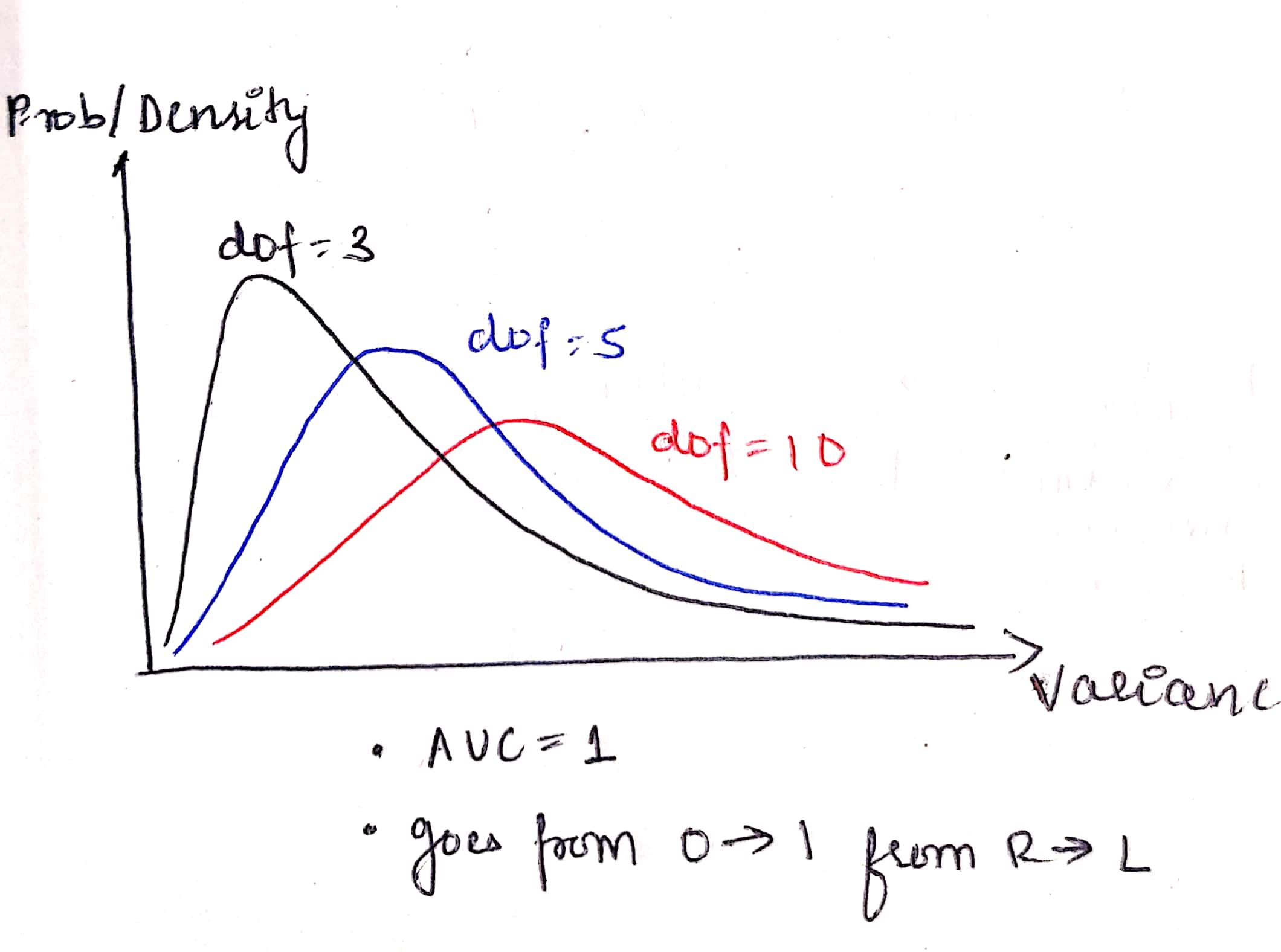
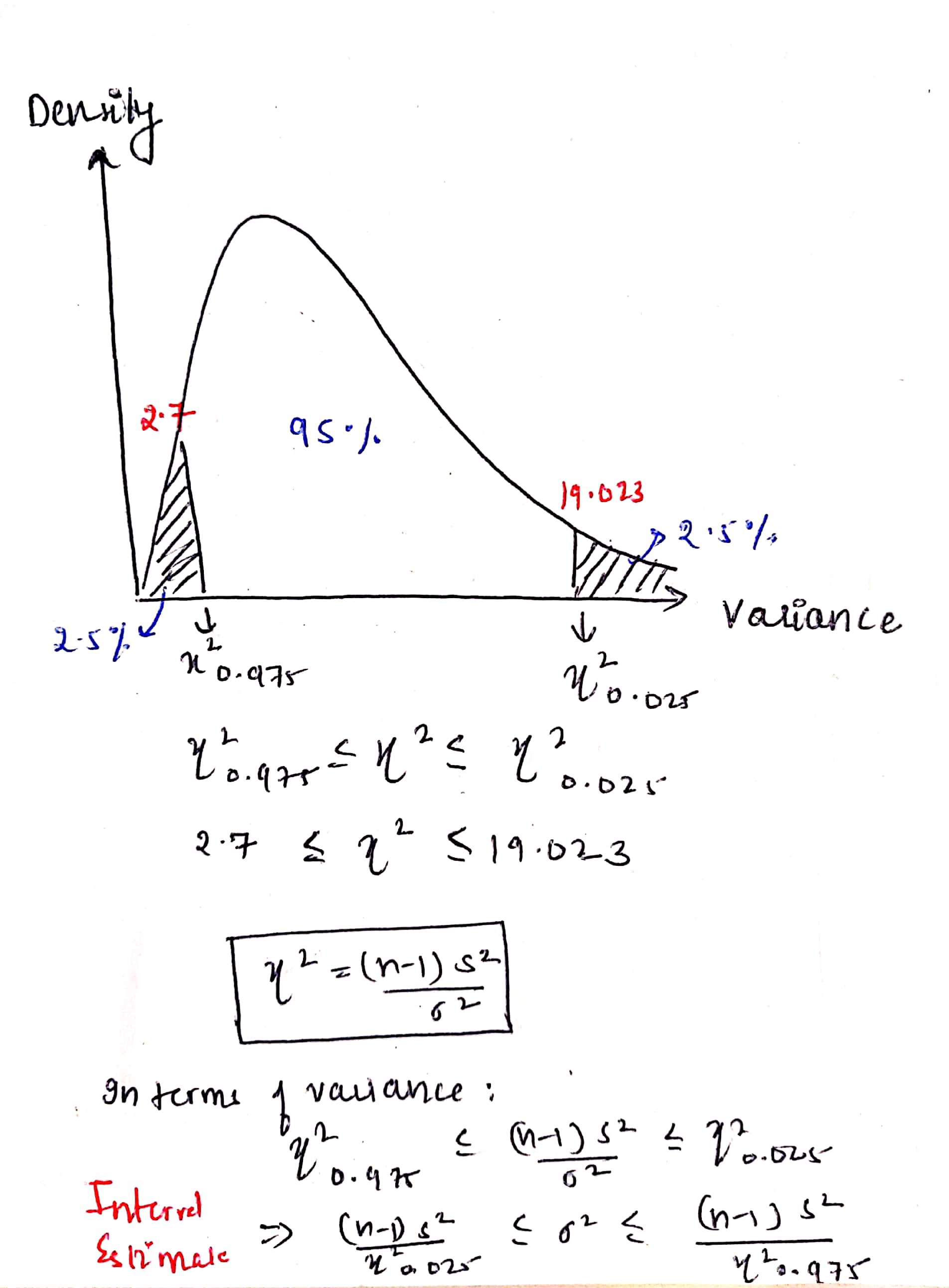
- distribution of sampling distribution of variances follow chi-square distribution
- chi-square distribution is not only ‘one’ and depends on alpha and dof (like t-distribution)
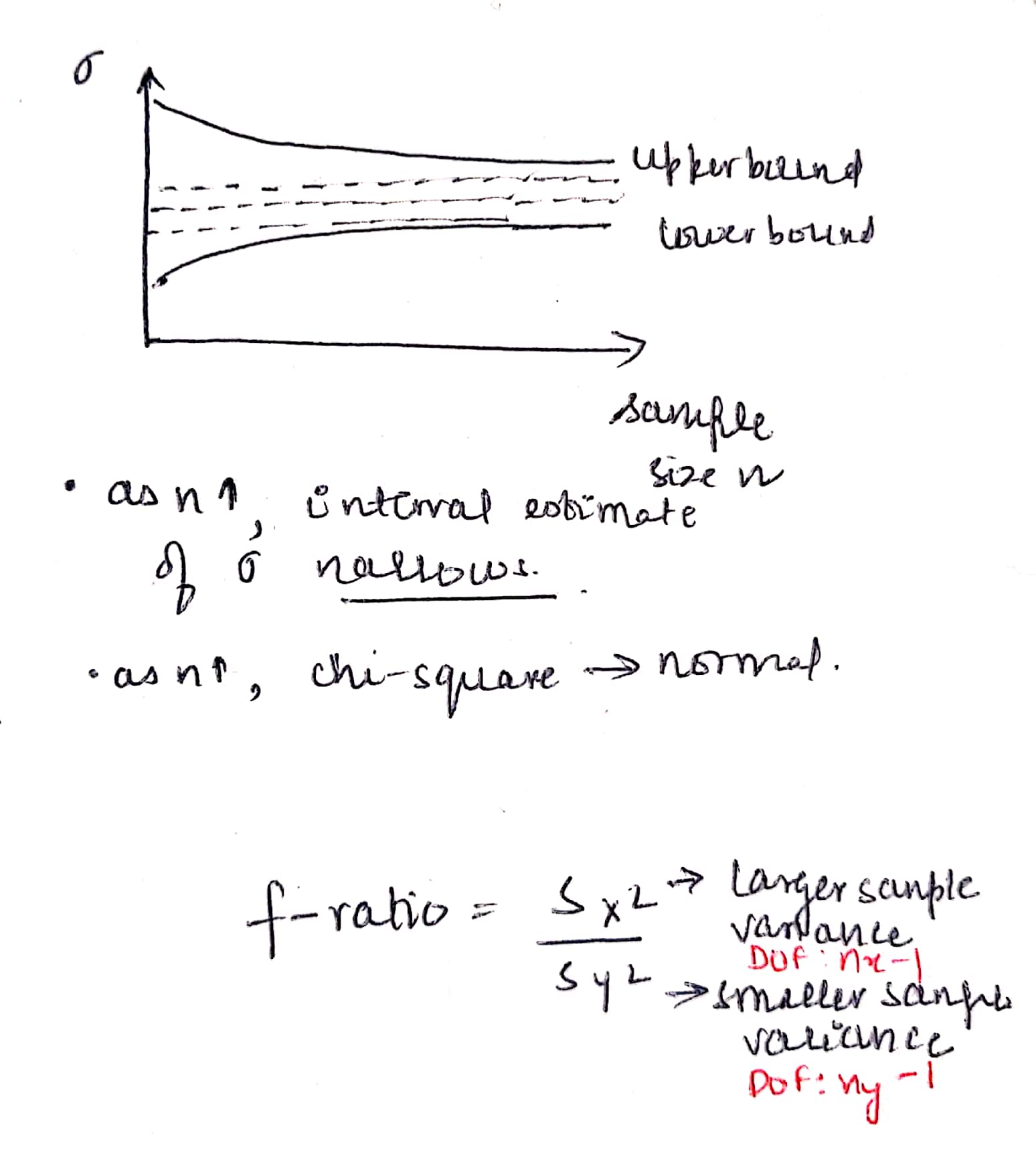
- as sample size n increases, the interval estimate of variance narrows and the chi-square distribution approaches normal distribution
 {width= 200px}
 {width=200 px}
 {width=200 px}
- Hypothesis testing of variance
- goal is to test whether a sample variance meets the assumption of hypothesized variance or not
- same process as above except the test-statistic and sampling distribution
- Types of hypothesis tests for variance:
- single sample hypothesis test: to check whether population variance is equal to hypothesized mean
- 3 types: two-tailed, right-tailed, left-tailed (extremely rare)
- two population hypothesis test: k/a f-ratio test to check whether variances of two populations are statistically different or not
- f-distribution : when independent random samples of two normal population are taken, the sampling distribution of the ratio of those sample variances follows f-distribution
- has two types of DOF: one for each population
- only right-tailed because either the variances are equal (null) or the Nr. one is larger than Dr. one (alternate)
- Chi-square test: test of independence
- to understand te relatonship between two categorical variables
- to test whether the co-variation between two variables is due to some random chance or there exists some important reltionship
- we get two contigency tables - OBSERVED and EXPECTED, to test the relationship between 2 variables. Ex. Student levels and years.
- chi-square test is done on the difference between observed and expected to check whether the difference is statistically significant or just random chance
- ANOVA
- to compare means of more than 2 populations; the point is to ask whether the populations come from the same overall population
- multiple t-tests do not work because it leads to compounding of error
- anova is a variability ratio = variance between/variance within
- total variance = variance between + variance within
- 3 cases:
- if ratio is large/small => reject Ho (Ho is all the populations come from same overall population)
- if ratio is similar/similar => fail to reject Ho
- if ratio is small/large => fail to reject Ho
- 2 types off anova : one-way adnd two-way
- in anova, we measure variance using sum of squares
- one-way:
- SST (total) = SSC (columns/between) + SSE (error/within)
- if SSC > SSE => reject Ho, there exists a difference
- two-way (also called Randomized Design):
- we add one more factor at the row level
- this helps in further untangle variance sources to make sure that the column variance is not masked by any other factor
- SST = SSC (columns) + SSB (blocks/rows) + minimized SSE (error)
- if SSC > minimized SSE => reject Ho, there exists a difference
- two-way with replication : 1) 2 factors 2) multiple measurements for each factor combination
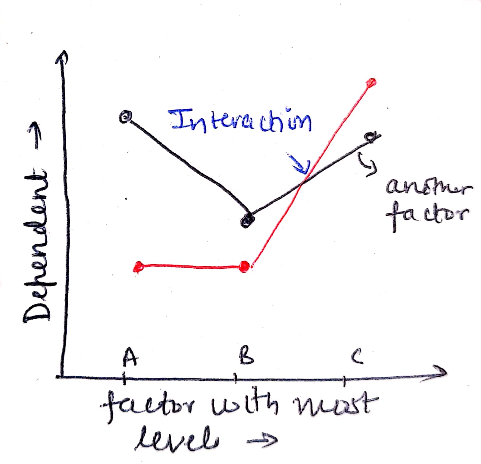
- Marginal Mean Graph (MMG)
- Interaction occurs when the effect of one factor changes for different levels of the other factor
- while reading ANOVA table, always look for interaction first. If interaction is significant, then the effect of each factor cannot be analyzed because they are too intertwined
keywords
ghjghgfhgf